[CS229] Lecture 3 Notes - LWR/Prob Interp/Logistic/Perceptron

Feb. 12, 2019 - Tuesday

Notes

cs229

machine learning

Locally Weighted Regression

Probablistic Interpretation of LR

Classification (Logistic Regression)

Disgression -> Perceptron

1. Locally Weighted Regression
2. Probablistic Interpretation of LR
3. Classification and Logistic Regression
- 3.1. Logistic regression for classification problems
4. Digression - Perceptron
Reference

1. Locally Weighted Regression

1.1. The origin:

The choice of features is important to ensuring good performance of a learning algorithm.
The Locally weighted linear regression (LWR) algorithm, which assuming there is sufficient training data, makes the choice of features less critical.

1.2. Detail:

The locally weighted linear regression alogorithm does the following:

Fit $ \theta $ to minimize $\sum_i w^{(i)} (y^{(i)} - \theta^T x^{(i)} )^2$.
Output $\theta^T x$.

where $w^{(i)} = \exp\left(-\frac{(x^{(i)} - x)^2}{2\tau^2}\right)$, $\tau$ is called “bandwidth”.

Note that:

the wights depend on the particular point $x$ at which we’re trying to evaluate $x$.
if $\vert x^{(i)} - x \vert$ is small, the $w^{(i)}$ is close to 1;
if $\vert x^{(i)} - x \vert$ is large, the $w^{(i)}$ is close to 0;

1.3. Parametric v.s. Non-Parametric Learning Algorighms:

“Parametric” learning algorithm:

Fix numbers of parameters to fit the model;

“Non-Parametric” learning algorithm:

Number of parameter grows with $m$ ($m$ is the training size).
To make predictions using LWR, we need to keep the entire training set around. (LWR is the first example in the class as a non-parametric algorithm).

2. Probablistic Interpretation of LR

2.1. Assumptions:

We assume that:

$y{(i)} = \theta^T x^{(i)} + \varepsilon^{(i)}$

where

$\varepsilon^{(i)}$ is the error and $\varepsilon^{(i)} \sim \mathcal{N}(0, \sigma^2)$, which means $P(\varepsilon^{(i)}) = \frac{1}{\sqrt{2\pi}\sigma}\exp\left(-\frac{(y^{(i)} - \theta^T x^{(i)})^2}{2\sigma^2}\right)$.
$\varepsilon^{(i)}$ is I.I.D. (independently identically distributed).

2.2. Maximum Likelihood

2.2.1. There are two different basic ideas in probability:

Frequency point of view -> (Applied here!)
Bayesian point of view.

2.2.2. The principle of maximum likelihood:

To choose $\theta$ to maximum $L(\theta)$, $\theta$ is NOT a random value, but a true value out there!

2.3. Find the best $\theta$ to reach the “Maximum Likelihood”:

Then, the “Likelihood” of the $y$ is:

$\begin{align} L(\theta) & = P\left(\mathbf{y} \vert X;\theta\right) \\ (i.i.d) & = \prod_{i=1}^m P\left(y^{(i)} \vert x^{(i)}; \theta\right) \\ & = \prod_{i=1}^m \frac{1}{\sqrt{2\pi}\sigma}\exp\left(-\frac{\left(y^{(i)} - \theta^T x^{(i)}\right)^2}{2\sigma^2}\right) \end{align}$

Then, for mathematical convenience, let

$\begin{align} l(\theta) &= \log\left(L(\theta)\right) \\ &= \log\left(\prod_{i=1}^m P\left(y^{(i)} \vert x^{(i)}; \theta\right)\right) \\ &= \sum_{i=1}^m \log P\left(y^{(i)} \vert x^{(i)}; \theta\right) \\ &= \sum_{i=1}^m \log\left(\frac{1}{\sqrt{2\pi}\sigma}\exp\left(-\frac{\left(y^{(i)} - \theta^T x^{(i)}\right)^2}{2\sigma^2}\right)\right) \\ &= m\cdot\log\frac{1}{\sqrt{2\pi}\sigma} + \sum_{i=1}^m \left(-\frac{\left(y^{(i)} - \theta^T x^{(i)}\right)^2}{2\sigma^2}\right). \end{align}$

Therefore, to maximize $l(\theta)$ is to minimize $\sum_{i=1}^m \frac{\left(y^{(i)} - \theta^T x^{(i)}\right)^2}{2\sigma^2}$, which is the same as minimizing $J(\theta) = \sum_{i=1}^m \frac{\left(y^{(i)} - \theta^T x^{(i)}\right)^2}{2}$ (this is the rule for Least Square).

3. Classification and Logistic Regression

Note: Generally, it’s bad idea to use LR for classification problems. Why? It doesn’t make sence for $h_\theta(x)$ to take values larger than 1 or smaller than 0 when we know that $y\in{0,1}$.

3.1. Logistic regression for classification problems

As in a classification problem:

$y \in \{0, 1\} \\ h_\theta(x) \in [0, 1]$

To fix the problems when using Linear Regression, we choose another form of function for our hypothesis $h_\theta(x)$.

$h_\theta(x) = g(\theta^Tx) = \frac{1}{1 + e^{-\theta^T x}},$

where

$g(z) = \frac{1}{1 + e^{-z}}.$

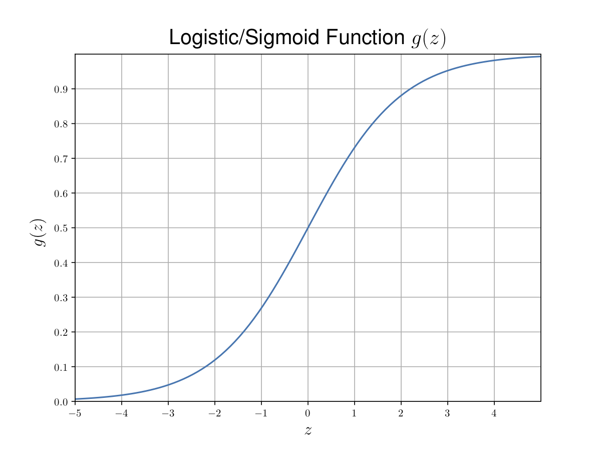
$g(z) = \frac{1}{1 + e^{-z}}$ is called “sigmoid” function or “logistic” function.


Figure 2. Sigmoid function.

Then, we have

$\left\{ \begin{array}{rcl} P(y=1 \vert x; \theta) & = & h_\theta(x) \\ P(y=0 \vert x; \theta) & = & 1 - h_\theta(x) \end{array}\right. \\ \Rightarrow P(y|x;\theta) = h_\theta(x)^y (1 - h_\theta(x))^{1-y}$

Then the likelihood is

$\begin{align} L(\theta) & = P\left(\mathbf{y} \vert X;\theta\right) \\ & = \prod_{i=1}^m P\left(y^{(i)} \vert x^{(i)}; \theta\right) \end{align}$

For mathematical convenience, let

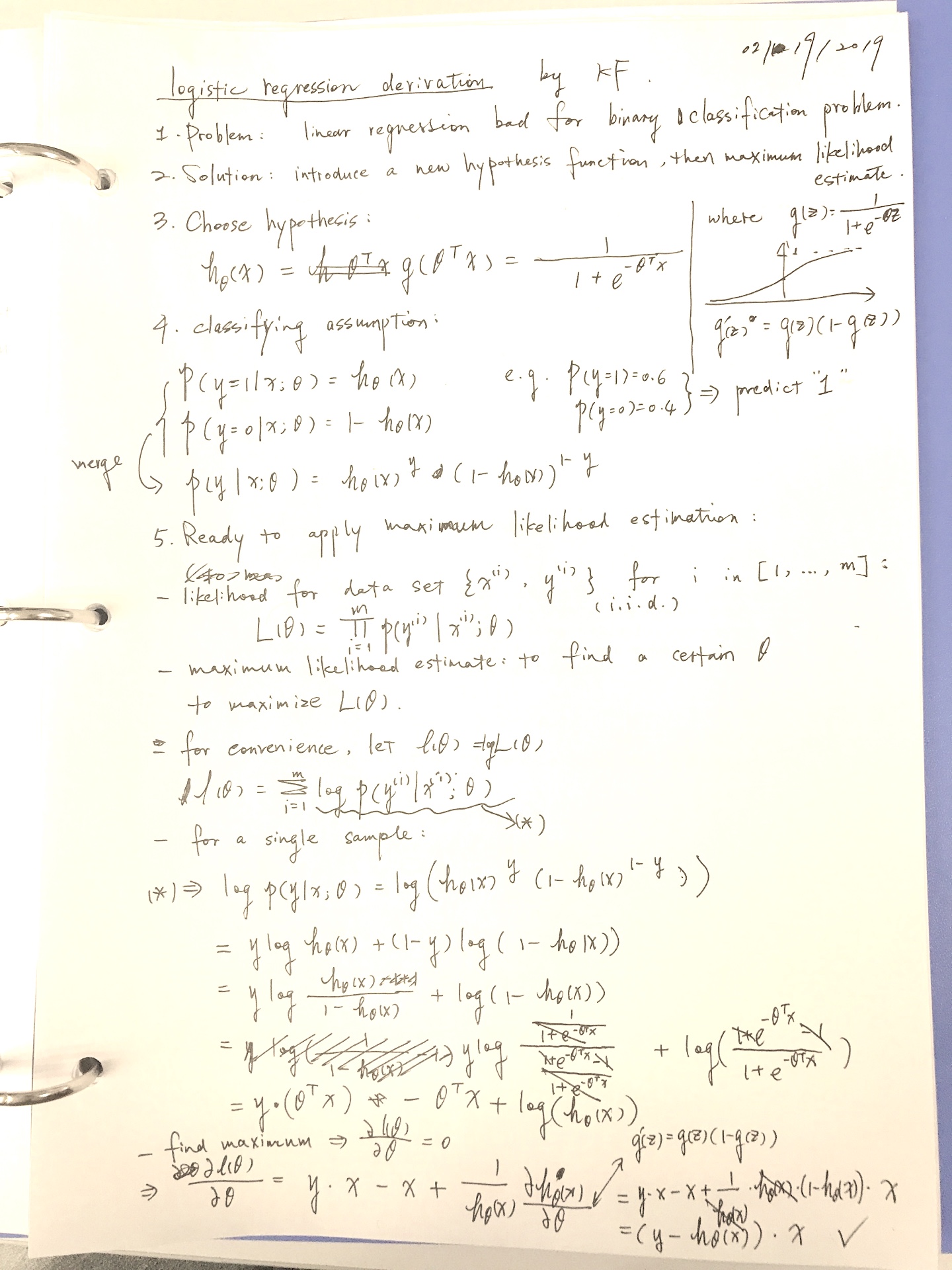
To maximize the likelihood, here we use gradient ascent by $\theta := \theta + \alpha \nabla_\theta l(\theta)$. The derivative is (derivation omitted, can be found on Page 18 in the notes):

$\frac{\partial}{\partial\theta_j}l(\theta) = \sum_{i=1}^m \left(y^{(i)} - h_\theta\left(x^{(i)}\right)\right)\cdot x_j^{(i)}$ $\theta_j := \theta_j + \alpha \sum_{i=1}^m \left(y^{(i)} - h_\theta\left(x^{(i)}\right)\right)\cdot x_j^{(i)}$

(added on 02/19/2019)


Note 1. Review of “logistic regression” from scratch.

4. Digression - Perceptron

Almost the same procedure as the logistic regression. The only difference is the $g(z)$ used in the process.

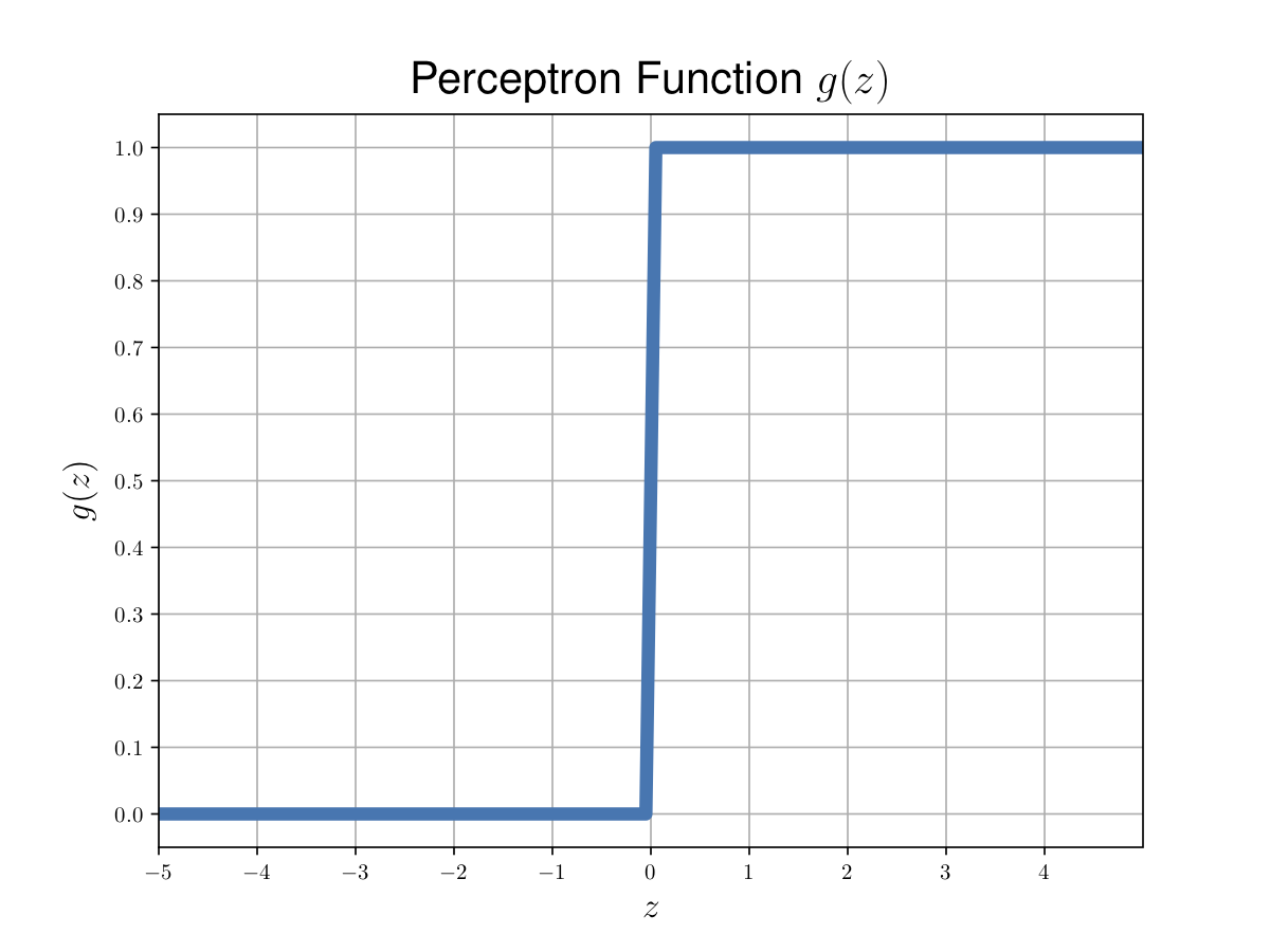
The $g(z)$ used in perceptron learning algorithm is:

$g(z) = \left\{ \begin{array}{rcl} 1 & \mbox{if} & z \ge 0 \\ 0 & \mbox{if} & z \lt 0 \end{array}\right.$


Figure 2. Perceptron function.

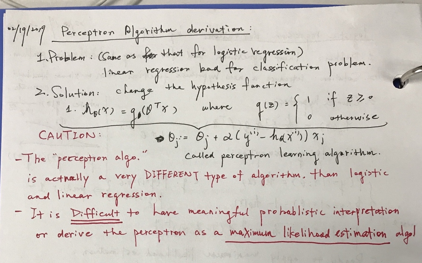
Then, $h_\theta(x) = g(\theta^T x)$, and the update rule for perceptron learning algorithm is almost the same:

$\theta_j := \theta_j + \alpha \left(y^{(i)} - h_\theta\left(x^{(i)}\right)\right)\cdot x_j^{(i)}$