[CS229] Lecture 5 Notes - Descriminative Learning v.s. Generative Learning Algorithm

Keep Updating:

• 2019-02-18 Merge to Lecture #5 Note
• 2019-01-23 Add Part 2, Gausian discriminant analysis
• 2019-01-22 Add Part 1, A Review of Generative Learning Algorithms.

• 1. Basics of Generative Learning Algorithms
  • 1.1. An Example to Explain the Initiative Ideas:
    • Approach I:
    • Approach II:
  • 1.2. Definitions:
    • Discriminative learning algorithms:
    • Generative learning algorithms:
  • 1.3. More about Generative Learning Algorithms:
• 2. Gaussian Discriminant Analysis (GDA)
  • 2.1. The multivariate normal distribution
  • 2.2. The Gaussian Discriminant Analysis model
    • (TO DO: Add the derivation)
    • Predict:
  • 2.3. GDA and logistic regression
    • Assumption relations:
    • Which is better?
• 3. Naive Bayes
  • Naive Bayes (NB) assumption:
  • Predict:
  • Laplace smoothing
• Reference

1. Basics of Generative Learning Algorithms

(01/22/2019)

1.1. An Example to Explain the Initiative Ideas:

Consider a classification problem in which we want to learn to distinguish between cats \((y=0)\) and dogs \((y=1)\):

Approach I:

Based on some features of an animal, given a training set, an algorithm like logistic regression or perceptron algorithm, tries to find a decision boundary (e.g. a straight line) to separate the cats and the dogs.

To classify a new animal:

Just check on which side of the decision boundary it falls.

Approach II:

First, look at cats, build a model of what cats look like. Then, look at dogs, build another model of what dogs look like.

To classify a new animal:

Match the new animal against the cat model and the dog model respectively, to see whether the new animal looks more like the cats or more like the dogs we had seen in the training set.

1.2. Definitions:

Discriminative learning algorithms:

Algorithms that try to learn \(p(y \vert x)\) directly (such as logistic regression) or algorithms that try to learn mappings directly from the space of input \(\chi\) to the labels \({0,1}\) (such as perceptron algorithm) are called discriminative learning algorithms.

Generative learning algorithms:

Algorithms that instead try to model \(p(x \vert y)\) and \(p(y)\) are called generative learning algorithms.

1.3. More about Generative Learning Algorithms:

Continue with the example of cats and dogs, if \(y\) indicates whether an sample is a cat (0) or a dog (1), then

• \(p(x \vert y=0)\) models the distribution of cats’ features.
• \(p(x \vert y=1)\) models the distribution of dogs’ features.

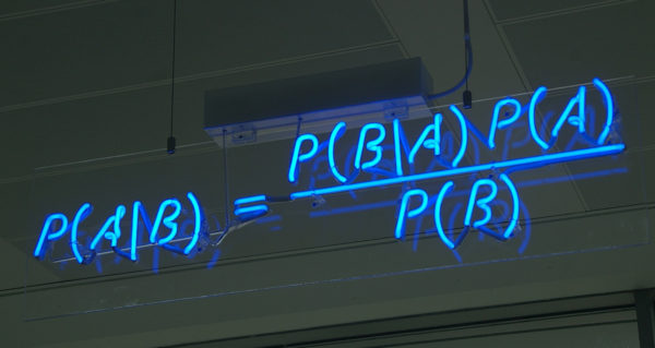
After modeling \(p(y)\) (called the class priors) and \(p(x \vert y)\), our algorithm can then use Bayes Rule to derive the posterior distribution on \(y\) given \(x\):

$$p(y \vert x) = \frac{p(x \vert y)p(y)}{p(x)}.$$

Here, the denominator is given by \(p(x)=\sum_i p(x \vert y_i)p(y_i)\). In cats & dogs example, \(p(x)=p(x \vert y=0)p(y=0)+p(x \vert y=1)p(y=1)\).

Actually, if we we’re calculating \(p(y \vert x)\) in order to make a prediction, then we don’t need to calculate the denominator, since

$$\begin{align} \arg\underset{y}{\max} p(y \vert x) & = \arg \underset{y}{\max} \frac{p(x \vert y)p(y)}{p(x)} \\ & = \arg \underset{y}{\max} p(x \vert y)p(y). \end{align}$$

2. Gaussian Discriminant Analysis (GDA)

(01/23/2019)

In this model (GDA), we assume that \(p(x \vert y)\) is distributed according to a multivariate normal distribution. First let’s talk briefly about the properties of multivariate normal distributions.

2.1. The multivariate normal distribution

The Definition of so-called multivariate normal distribution:

• A distribution with a mean vector \(\mu \in \mathbb{R}^n\) and a covariance matrix \(\Sigma \in \mathbb{R}^{n \times n}\), where \(\Sigma \geq 0\) is symmetric and positive semi-definite. Also written “\(\mathcal{N}(\mu, \Sigma)\)”, it’s density is given by:

$$p(x; \mu, \Sigma) = \frac{1}{(2\pi)^{n/2}|\Sigma|^{1/2}}\exp\left(-\frac{1}{2}(x-\mu)^T\Sigma^{-1}(x-\mu)\right).$$

where “\(\vert\Sigma\vert\)” denotes the determinant of the matrix \(\Sigma\).

• For a random variable \(X\) distributed \(\mathcal{N}(\mu, \Sigma)\), the mean is given by \(\mu\):

$$\text{E}[X] = \int_x x\ p(x;\mu,\Sigma)dx = \mu$$

• The covariance of a vector-valued random variable \(Z\) is defined as \(\text{Cov}(Z) = \text{E}[(Z-\text{E}[Z])(Z-\text{E}[Z])^T]\), which can also be written as \(\text{Cov}(Z) = \text{E}[ZZ^T]-(\text{E}[Z])(\text{E}[Z])^T\). If \(X \sim \mathcal{N}(\mu, \Sigma)\), then:

$$\text{Cov}(X) = \Sigma.$$

2.2. The Gaussian Discriminant Analysis model

(02/18/2019)

When $x$ are continuous-valued variables, we can use the so-called Gaussian Discriminant Analysis (GDA) which using multivariate normal distribution to model the different cases:

$$\begin{align} y &\sim \mbox{Bernoulli}(\phi) \\ x \vert y=0 &\sim \mathcal{N}(\mu_0, \Sigma) \\ x \vert y=1 &\sim \mathcal{N}(\mu_1, \Sigma) \end{align}$$

which can be written as:

$$\begin{align} p(y) &= \phi^y(1-\phi)^{1-y} \\ p(x\vert y=0) &= \frac{1}{(2\pi)^{n/2} \vert\Sigma\vert^{1/2}}\exp\left(-\frac{1}{2}(x-\mu_0)^T\Sigma^{-1}(x-\mu_0)\right) \\ p(x\vert y=1) &= \frac{1}{(2\pi)^{n/2} \vert\Sigma\vert^{1/2}}\exp\left(-\frac{1}{2}(x-\mu_1)^T\Sigma^{-1}(x-\mu_1)\right) \end{align}$$

Now the parameters are: $\phi, \mu_0, \mu_1, \Sigma$. Apply maximum likelihood estimate, the log-likelihood would be:

$$\begin{align} l(\phi, \mu_0,\mu_1,\Sigma) &= \log\prod_{i=1}^m p(x^{(i)}, y^{(i)}; \phi,\mu_0,\mu_1,\Sigma) \\ &= \log\prod_{i=1}^m p(x^{(i)} \vert y^{(i)};\mu_0,\mu_1,\Sigma)p(y^{(i)};\phi) \end{align}$$

(TO DO: Add the derivation)

We get the maximum likelihood estimate of these parameters:

$$\begin{align} \phi &= \frac{1}{m} \sum_{i=1}^m 1\{ y^{(i)}=1 \} \\ \mu_0 &= \frac{\sum_{i=1}^m 1\{ y^{(i)}=0 \} x^{(i)}}{\sum_{i=1}m 1\{ y{(i)}=0 \}} \\ \mu_1 &= \frac{\sum_{i=1}^m 1\{ y^{(i)}=1 \} x^{(i)}}{\sum_{i=1}m 1\{ y{(i)}=1 \}} \\ \Sigma &= \frac{1}{m}\sum_{i=1}^m (x^{(i)} - \mu_{y^{(i)}})(x^{(i)} - \mu_{y^{(i)}})^T. \end{align}$$

Predict:

Simply apply the rules mentioned above, with these estimates:

$$\begin{align} \arg\underset{y}{\max} p(y \vert x) & = \arg \underset{y}{\max} \frac{p(x \vert y)p(y)}{p(x)} \\ & = \arg \underset{y}{\max} p(x \vert y)p(y). \end{align}$$

2.3. GDA and logistic regression

With the predicting rules above, we have:

$$p(y=1 vert x;\phi,\Sigma,\mu_0,\mu_1) = \frac{1}{1 + \exp(-\theta^Tx)}.$$

where $\theta$ is some appropriate function of $\phi,\Sigma,\mu_0,\mu_1$. This is exactly the form that logistic regression, a discriminative algorithm, to model $p(y=1 \vert x)$.

Assumption relations:

$\begin{align} p(x \vert y) \text{ is multivariate gaussian} &\Rightarrow p(x \vert y) \text{ follows a logistic function/ExpFamily} \\ p(x \vert y) \text{ is multivariate gaussian} &\nLeftarrow p(x \vert y) \text{ follows a logistic function/ExpFamily} \\ \end{align}$

Which is better?

• When $p(x \vert y)$ is really Gaussian, GDA is asymptotically efficient!
• By making weaker assumptions logistic regression is more robust, especially the data is indeed non-Gaussian, then in the limit of large datasets, logistic regression will almost always do better than GDA. For this reason, in practice logistic regression is used more often than GDA.

3. Naive Bayes

(02/18/2019)

As GDA is for continuous $x$ problems, here Naive Bayes is for those problems with discrete $x$.

Here’s the typical example: spam filter.

First, we present the email(text) via a feature vector whose length is the size of word dictionary (a fixed number). If the email contains the $j$-th word, $x_j=1$; otherwise $x_j=0$. The vector would like like this:

$$\begin{align} x = \left[\begin{array}{c} 1\\0\\0\\\vdots\\1\\\vdots\\0 \end{array}\right] \quad \begin{array}{l} \text{a}\\\text{aardvark}\\\text{aardwolf}\\\vdots\\\text{buy}\\\vdots\\\text{zygmurgy}\end{array} \\ \end{align}$$

If our vocabulary size is 50000, then $x \in \{ 0, 1 \}^{50000}$ ($x$ is a 50000-dimensional vector of 0’s and 1’s). If we were to model $x$ discriminatively/explicitly with multinomial distribution over the $2^{50000}$ possible outcomes, the we’d end up with a ($2^{50000} -1$)-dimensional parameter vector, which is not appliable.

Naive Bayes (NB) assumption:

• To model $p(x \vert y)$, we have to assume that the $x_i$’s are conditionally independent given $y$.
• Under such assumption, the resulting algorithm is called the Naive Bayes classifier.

Then, we have:

$$\begin{align} & p(x_1,\dots,x_{50000} \vert y) \\ &= p(x_1 \vert y)p(x_2 \vert y, x_1)p(x_3 \vert y, x_1,x_2)\cdots p(x_{50000}\vert y,x_1,\dots,x_{49999}) \\ &= p(x_1\vert y)p(x_2\vert y)p(x_3\vert y)\cdots p(x_{50000}\vert y) \\ &= \prod_{j=1}^n p(x_j\vert y) \end{align}$$

Our model now is parameterized by:

$$\left\{ \begin{array}{rcl} \phi_{j\vert y=1} &= &p(x_j=1\vert y=1) \\ \phi_{j\vert y=0} &= &p(x_j=1\vert y=0) \\ \phi_y &= &p(y=1) \end{array} \right.$$

The likelihood of the data:

$$\mathcal{L}(\phi_y,\phi_{j\vert y=0},\phi_{j\vert y=1}) = \prod_{i=1}^m p(x^{(i)}, y^{(i)}).$$

Then we can get the maximum likelihood estimates:

$$\begin{align} \hat\phi_{j\vert y=1} &= \frac{\sum_{i=1}^m 1\{x_j^{(i)} =1 \wedge y^{(i)} = 1 \}}{\sum_{i=1}^m 1\{y^{(i)} = 1 \}} \\ \hat\phi_{j\vert y=0} &= \frac{\sum_{i=1}^m 1\{x_j^{(i)} =1 \wedge y^{(i)} = 0 \}}{\sum_{i=1}^m 1\{y^{(i)} = 0 \}} \\ \hat\phi_y &= \frac{\sum_{i=1}^m 1\{y^{(i)} = 1\}}m \end{align}$$

In the equation above, the “$\wedge$” symbol means “and”. The estimates have a very natural interpretation. For instance, $\phi_{j\vert y=1}$ is just the fraction of spam $(y=1)$ emails in which word $j$ does appear.

Predict:

To make a prediction on a new sample with feature $x$, we then simply calculate:

$$\begin{align} p(y=1\vert x) &= \frac{p(x\vert y=1)p(y=1)}{p(x)} \\ &= \frac{\left(\prod_{j=1}^n p(x_j\vert y=1)\right)p(y=1)}{\prod_{j=1}^n p(x_j\vert y=1)p(y=1) + \prod_{j=1}^n p(x_j\vert y=0)p(y=0)} \end{align}$$

and pick the class has the higher posterior probability.

Laplace smoothing

Here is a problem:

• If there is a new word ($k$-th in the dictionary) appeared in the email text, which is not included in you training set. Then,

$$\prod_{j=1}^n p(x_j\vert y=1) = 0\Leftarrow p(x_k\vert y=1) = 0\\ \prod_{j=1}^n p(x_j\vert y=0) = 0 \Leftarrow p(x_k\vert y=1) = 0$$

Then,

$$\begin{align} p(y=1\vert x) &= \frac{\left(\prod_{j=1}^n p(x_j\vert y=1)\right)p(y=1)}{\prod_{j=1}^n p(x_j\vert y=1)p(y=1) + \prod_{j=1}^n p(x_j\vert y=0)p(y=0)} \\ &= \frac0{0}. \end{align}$$

To avoid this, we introduce Laplace smoothing, which replace the estimate with:

$$\phi_j = \frac{\sum_{i=1}^m 1 \{z^{(i)} \} + 1}{m+k}.$$

Then the estimates is updated as:

$$\begin{align} \hat\phi_{j\vert y=1} &= \frac{\sum_{i=1}^m 1\{x_j^{(i)} =1 \wedge y^{(i)} = 1 \} + 1 }{\sum_{i=1}^m 1\{y^{(i)} = 1 \} + 2 } \\ \hat\phi_{j\vert y=0} &= \frac{\sum_{i=1}^m 1\{x_j^{(i)} =1 \wedge y^{(i)} = 0 \} + 1 }{\sum_{i=1}^m 1\{y^{(i)} = 0 \} + 2 } \end{align}$$

Note: In practice, it usually doesn’t matter much whether we apply Laplace smoothing to $\phi_y$ or not, since we will typically have a fair fraction each of spam and non-spam message, so $\phi_y$ will be a reasonable estimate of $p(y=1)$ and will be quite far from 0 anyway. WHY?

Reference

1. » Stanford CS229 Lecture Note Part IV - Generative Learning Algorithms

KF