[CS229] Lecture 4 Notes - Newton's Method/GLMs

1. Newton’s Method,
2. Generalized Linear Models

• 1. Newton’s Method
  • 1.1. Basic idea of Newton’s method
  • 1.2. Use Newton’s method to maximize some function \(l\)
  • 1.3. Pros & Cons of Newton’s method
• 2. Generalized Linear Models
  • 2.1. The exponential family
    • 2.1.1. Bernoulli case
    • 2.1.2. Gaussian case
• 3. Constructing GLMs
  • 3.1. Ordinary Least Squares
  • 3.2. Logistic Regression
  • 3.3. Softmax Regression
• Reference

1. Newton’s Method

1.1. Basic idea of Newton’s method

The aim of Newton’s method is to find a zero of a function.

Suppose we have some function that \(f: \mathbb{R}\mapsto\mathbb{R}\), and we want to find a value of \(x\) that makes \(f(x)=0\). Newton’s method performs the following updates:

$$x := x - \frac{f(x)}{f'(x)}.$$

» Newton’s Method on Wikipedia

Figure 1. The function \(f\) is shown in blue and the tangent line is in red. We see that \(x_{n + 1}\) is a better approximation than \(x_n\) for the root x of the function \(f\). (from Wikipedia)

1.2. Use Newton’s method to maximize some function \(l\)

The maxima of \(l\) correspond to points where it’s first derivative \(l’(\theta)\) is zero. Therefore, according to the definition of Newton’s method described above, to find a value of \(\theta\) that makes \(f’(\theta)=0\), we should perform the following update:

$$\theta := \theta - \frac{f'(\theta)}{f''(\theta)}.$$

In the logistic regression, \(\theta\) is a vector, then the update rule should be generalized as:

$$\theta := \theta - H^{-1}\nabla_\theta l(\theta).$$

Here \(\nabla_\theta l(\theta)\) is the vector of partial derivatives of \(l(\theta)\) w.r.t. the \(\theta\)’s; and the \(H\) is an n-by-n matrix called Hessian, whose entries are given by

$$H_{ij} = \frac{\partial^2 l(\theta)}{\partial\theta_i\partial\theta_j}.$$

1.3. Pros & Cons of Newton’s method

Pros:

• Newton’s method converges faster that gradient descent and requires fewer iterations to get close to the minimum.

Cons:

• Each single iteration however is more expensive that the one of gradient descent, since it requires finding and inverting an n-by-n Hessian.

2. Generalized Linear Models

Both linear regression and logistic regression methods are special cases of a broader family of models, which is called Generalized Linear Models (GLMs).

2.1. The exponential family

Define a class of distributions in the exponential family as:

$$\begin{align} p(y;\eta) = b(y)\exp(\eta^T T(y) - a(\eta)). \tag{*}\label{eq1} \end{align}$$

• \(\eta\) - is called the natural parameter of the distribution;
• \(T(y)\) - is the sufficient statistic;
• \(a(\eta)\) - is the log partition function.

A family:

• A fixed choice of \(T\), \(a\) and \(b\) defines a family of distributions that is parameterized by \(\eta\).
• As we vary \(\eta\), we could get different distributions within this family.

We’ll show that the Bernoulli and the Gaussian distributions are examples of exponential family distributions.

2.1.1. Bernoulli case

The Bernoulli distribution with mean \(\phi\), written Bernoulli\((\phi)\), specifies a distribution over \(y \in {0,1}\). So that

$$\left\{ \begin{array}{rcl} P(y=1;\phi) &=& \phi \\ P(y=0;\phi) &=& 1-\phi \end{array}\right. \\ $$

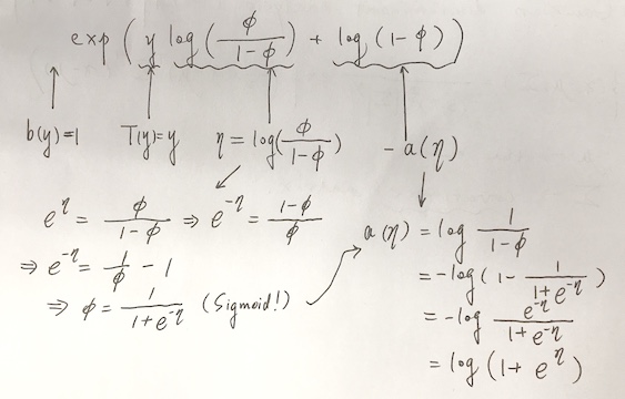
This class of distributions is parameterized by \(\phi\). Now we want to show that this class of Bernoulli distributions is in the “exponential family” when we choose a certain set of \(T\), \(a\) and \(b\). We write the Bernoulli distribution as:

$$\begin{align} p(y;\phi) &= \phi^y(1-\phi)^{1-y} \\ &= \exp(\log(\phi^y(1-\phi)^{1-y}) \\ &= \exp(y\log\phi + (1-y)\log(1-\phi)) \\ &= \exp(y\log\phi -y\log(1-\phi) + log(1-\phi)) \\ &= \exp\left(y\log\frac{\phi}{1-\phi} + \log(1-\phi)\right). \end{align}$$

according to Equation \(\eqref{eq1}\), we do the following derivation:

Figure 2. Derivation of Bernoulli to GLM

We have

$$\begin{align} \eta &= \log\frac{\phi}{1-\phi} \\ T(y) &= y \\ a(\eta) &= \log(1+e^\eta) \\ b(y) &= 1 \end{align}$$

This shows that the Bernoulli distribution can be written in the form of Equation \(\eqref{eq1}\), using certain choice of \(T\), \(a\) and \(b\) above.

2.1.2. Gaussian case

When deriving linear regression, the value of $\sigma^2$ had no effect on the choice of $\theta$ and $h_\theta(x)$. Thus, for simplicity, we set $\sigma^2=1$. Then for the Gaussian distribution, we have:

$$\begin{align} p(y;\mu) &= \frac{1}{\sqrt{2\pi}}\exp\left(-\frac{1}{2}(y-\mu)^2\right) \\ &= \frac{1}{\sqrt{2\pi}}\exp\left(-\frac{1}{2}y^2\right)\cdot\exp\left(y\mu-\frac{1}{2}\mu^2\right) \end{align}$$

Figure 3. Derivation of Gaussian to GLM

We have

$$\begin{align} \eta &= \mu \\ T(y) &= y \\ a(\eta) &= \frac{1}{2}\mu^2=\frac{1}{2}\eta^2 \\ b(y) &= \frac{1}{\sqrt{2\pi}}\exp\left(-\frac{1}{2}y^2\right). \end{align}$$

There are a lot of other distributions that belong to the exponential family, such as:

• the multinomial;
• the Poisson (for modelling count-data);
• the gamma and the exponential (for modelling continuous, non-negative random variables, such as time-intervals);
• the beta and the Dirichlet (for distributions over probabilities).

3. Constructing GLMs

Consider a classification or regression problem where we’d like to predict the value of some random variable $y$ as a function of $x$. To derive a GLM for this problem, we will make 3 assumptions about the conditional distribution of $y$ given $x$:

1. $y \vert x; \theta \sim \text{ExponentialFamily}(\eta)$. i.e., given $x$ and $\theta$, the distribution of $y$ follows some exponential family distribution with parameter $\eta$.
2. We would like the prediction $h(x)$ output to satisfy $h(x) = \mbox{E}[y\vert x]$. Why?
3. $\eta$ and $x$ should be linearly related: $\eta=\theta^T x$.(or if $\eta$ is a vector, then $\eta_i=\theta_i^T x$).

3.1. Ordinary Least Squares

3.2. Logistic Regression

3.3. Softmax Regression

Reference

1. » Stanford Lecture Note Part I & II

KF