[Python/NumPy] Matrix(Arrays) Manipulations & Operations
-
date_range Feb. 28, 2019 - Thursday info
A collection of frequently used python/numpy techniques on matrix (numpy arrays) manipulation and operations.

- 1. Indexing and Slicing
- 2. Numerical operations on arrays
- Reference
1. Indexing and Slicing
1.1. np.may_share_memory(), check array same in memory or not:
A slicing operation creates a view on the original array, which is just a way of accessing array data. Thus the original array is not copied in memory. You can use np.may_share_memory() to check if two arrays share the same memory block. Note however, that this uses heuristics and may give you false positives.
When modifying the view, the original array is modified as well:
>>> a = np.arange(10)
>>> a
array([0, 1, 2, 3, 4, 5, 6, 7, 8, 9])
>>> b = a[::2]
>>> b
array([0, 2, 4, 6, 8])
>>> np.may_share_memory(a, b)
True
>>> b[0] = 12
>>> b
array([12,  2,  4,  6,  8])
>>> a   # (!)
array([12,  1,  2,  3,  4,  5,  6,  7,  8,  9])

>>> a = np.arange(10)
>>> c = a[::2].copy()  # force a copy
>>> c[0] = 12
>>> a
array([0, 1, 2, 3, 4, 5, 6, 7, 8, 9])

>>> np.may_share_memory(a, c)
False
1.2. Fancy Indexing
NumPy arrays can be indexed with slices, but also with boolean or integer arrays (masks). This method is called fancy indexing. It creates copies not views.
1.2.1. Using boolean masks - a[mask]
>>> a = np.arange(20)
>>> a[a % 3 == 0]       # fancy indexing using boolean masks
array([ 0,  3,  6,  9, 12, 15, 18])

>>> b = a[a % 3 == 0]
>>> np.may_share_memory(a, b)  # prove that it's a copy not a view!
False

>>> a % 3 == 0          # generate a boolean mask
array([ True, False, False,  True, False, False,  True, False, False,
        True, False, False,  True, False, False,  True, False, False,
        True, False])

>>> mask = (a % 3 == 0)
>>> c = a[mask]         # fancy indexing using the mask (same way)
>>> c
array([ 0,  3,  6,  9, 12, 15, 18])
Indexing with a mask can be very useful to assign a new value to a sub-array:
>>> a = np.arange(20)
>>> a[a % 3 == 0] = -1
>>> a
array([-1,  1,  2, -1,  4,  5, -1,  7,  8, -1, 10, 11, -1, 13, 14, -1, 16, 17, -1, 19])
1.2.2. Indexing with an array of integers - a[list]
>>> a = np.arange(10)*100
array([  0, 100, 200, 300, 400, 500, 600, 700, 800, 900])

>>> b = [2, 4, 3, 3]
>>> a[b]
array([200, 400, 300, 300])
2. Numerical operations on arrays
2.1. Elementwise operations
2.1.1. Basic operations
All arithmetic operates (+, -, *, /, **, ...) elementwise:
These operations are of course much faster than if you did them in pure python:
# Test NumPy elementwise op efficiency
>>> a = np.arange(10000)
>>> %timeit a + 1
10000 loops, best of 3: 24.3 us per loop
>>> l = range(10000)
>>> %timeit [i+1 for i in l]
1000 loops, best of 3: 861 us per loop
2.1.2. Other operations
Comparisons:
>>> a = np.array([1, 2, 3, 4])
>>> b = np.array([4, 2, 2, 4])
>>> a == b
array([False,  True, False,  True], dtype=bool)
>>> a > b
array([False, False,  True, False], dtype=bool)
Array-wise comparisons:
>>> a = np.array([1, 2, 3, 4])
>>> b = np.array([4, 2, 2, 4])
>>> c = np.array([1, 2, 3, 4])
>>> np.array_equal(a, b)
False
>>> np.array_equal(a, c)
True
Logical operations:
>>> a = np.array([1, 1, 0, 0], dtype=bool)
>>> b = np.array([1, 0, 1, 0], dtype=bool)
>>> np.logical_or(a, b)
array([ True,  True,  True, False], dtype=bool)
>>> np.logical_and(a, b)
array([ True, False, False, False], dtype=bool)
Transcendental functions: (what’s transcendental functions”?)
>>> a = np.arange(5)
>>> np.sin(a)
array([ 0.        ,  0.84147098,  0.90929743,  0.14112001, -0.7568025 ])
>>> np.log(a)
array([       -inf,  0.        ,  0.69314718,  1.09861229,  1.38629436])
>>> np.exp(a)
array([  1.        ,   2.71828183,   7.3890561 ,  20.08553692,  54.59815003])
2.2. Reductions (sum, max, argmax, mean, median, std, any, all,…)
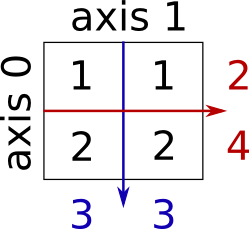
Reduction - Rule of Thumb: the result shape should be the original shape get the dimension (added as argument
axis=*in the op function) removed!(e.g.) a.shape -> (2,3,4), then:
- op(axis=0),the result shape should be (3,4) (axis 0, ‘2’ removed).
- op(axis=1),the result shape should be (2,4) (axis 1, ‘3’ removed).
- op(axis=2),the result shape should be (2,3) (axis 2, ‘4’ removed).
 |
|---|
| Figure 1. description of axis direction. |
# Reduction
>>> a = np.arange(24).reshape(2,3,4)
>>> a
array([[[ 0,  1,  2,  3],
        [ 4,  5,  6,  7],
        [ 8,  9, 10, 11]],

       [[12, 13, 14, 15],
        [16, 17, 18, 19],
        [20, 21, 22, 23]]])

# 1. Sum
>>> a.sum(axis=0)
array([[12, 14, 16, 18],
       [20, 22, 24, 26],
       [28, 30, 32, 34]])
>>> a.sum(axis=1)
array([[12, 15, 18, 21],
       [48, 51, 54, 57]])
>>> a.sum(axis=2)
array([[ 6, 22, 38],
       [54, 70, 86]])

# 2. Extrema: (min, max, argmin, argmax)
>>> a.min(axis=1)
array([[ 0,  1,  2,  3],
       [12, 13, 14, 15]])
>>> a.max(axis=2)
array([[ 3,  7, 11],
       [15, 19, 23]])
>>> a.argmax(axis=0)
array([[1, 1, 1, 1],
       [1, 1, 1, 1],
       [1, 1, 1, 1]])

# 3. Logical operations:
>>> a.all(axis=0)
array([[False,  True,  True,  True],
       [ True,  True,  True,  True],
       [ True,  True,  True,  True]])
>>> a.any(axis=2)
array([[ True,  True,  True],
       [ True,  True,  True]])

# 4. Statistics:
#   mean:
>>> a.mean(axis=1)
array([[ 4.,  5.,  6.,  7.],
       [16., 17., 18., 19.]])
#   median:
>>> np.median(a, axis=2)
array([[ 1.5,  5.5,  9.5],
       [13.5, 17.5, 21.5]])
#   std:
>>> a.std(axis=0)
array([[6., 6., 6., 6.],
       [6., 6., 6., 6.],
       [6., 6., 6., 6.]])
>>> a
array([[[ 0,  1,  2,  3],
        [ 4,  5,  6,  7],
        [ 8,  9, 10, 11]],

       [[12, 13, 14, 15],
        [16, 17, 18, 19],
        [20, 21, 22, 23]]])
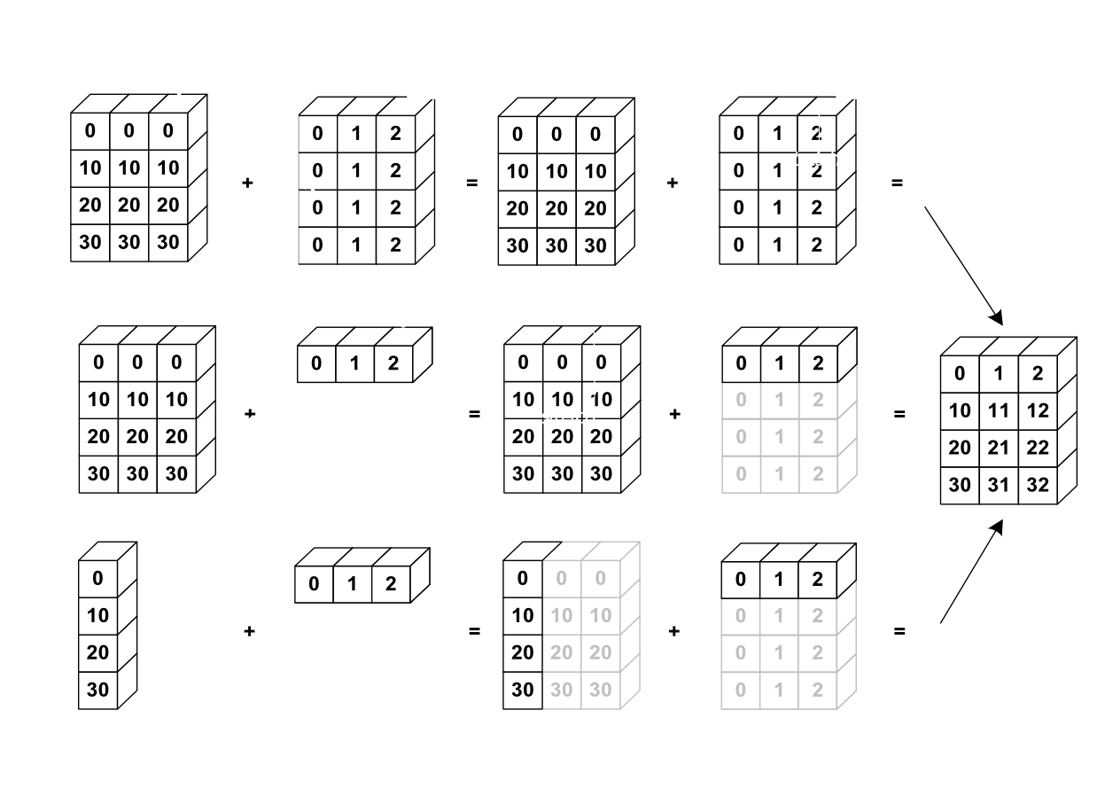
2.3. Broadcasting (PRETTY COOL!)
Definition of “Broadcasting”:
- It is possible to do operations on “different-size” arrays if Numpy can transform them into same size. This transformation is call “Broadcasting”.
 |
|---|
| Figure 2. Numpy broadcasting rule representation. |
# Broadcasting example 1:
>>> a                       # shape: (2,3)
array([[0, 1, 2],
       [3, 4, 5]])
>>> b                       # shape: (2,1)
array([[10.],
       [10.]])
>>> c                       # shape: (1,3)
array([[20., 20., 20.]])
>>> a + b
array([[10., 11., 12.],
       [13., 14., 15.]])
>>> a + c
array([[20., 21., 22.],
       [23., 24., 25.]])
>>> b + c
array([[30., 30., 30.],
       [30., 30., 30.]])

# Broadcasting example 2:
>>> a = np.arange(5)
>>> b = np.arange(3)[:,None]
>>> a
array([0, 1, 2, 3, 4])      # shape: (5,)
>>> b                       # shape: (3,1)
array([[0],
       [1],
       [2]])
>>> a + b
array([[0, 1, 2, 3, 4],
       [1, 2, 3, 4, 5],
       [2, 3, 4, 5, 6]])
2.4. Array Shape Manipulation
2.4.1. Reshape and Flattening (np.reshape, np.ravel, np.ndarray.flatten)
np.reshapeis simple, you can undertand it as a reverse operation of flattening.
As for flattening, there are several ways (difference in brief from StackOverflow):
np.ravel(usually faster, returns a view of the original array whenever possible.)np.ndarray.flatten(always returns a copy.)reshape((-1,))(gets a view whenever the strides of the array allow it even if that means you don’t always get a contiguous array.)
2.4.2. Add Dimension to Array
There are several ways to work it out, the results are the same:
- simply use
None; - apply
np.newaxis(actually,np.newaxisisNone); - use function:
np.expand_dims.
>>> a
array([[0, 1, 2],
       [3, 4, 5]])
>>> a[None,:]
array([[[0, 1, 2],
        [3, 4, 5]]])
>>> a[np.newaxis,:]
array([[[0, 1, 2],
        [3, 4, 5]]])
>>> np.expand_dims(a, axis=0)
array([[[0, 1, 2],
        [3, 4, 5]]])
2.4.3. Dimension shuffling (np.transpose)
>>> a = np.arange(4*3*2).reshape(4, 3, 2)
>>> a.shape
(4, 3, 2)
>>> a[0, 2, 1]
5
>>> b = a.transpose(1, 2, 0)
>>> b.shape
(3, 2, 4)
>>> b[2, 1, 0]
5

# Also creates a view:
>>>
>>> b[2, 1, 0] = -1
>>> a[0, 2, 1]
-1
2.4.4. Resizing (np.resize)
Size of an array can be changed with ndarray.resize:
>>> a = np.arange(4)
>>> a.resize((8,))
>>> a
array([0, 1, 2, 3, 0, 0, 0, 0])
However, it must not be referred to somewhere else:
>>>
>>> b = a
>>> a.resize((4,))
Traceback (most recent call last):
  File "<stdin>", line 1, in <module>
ValueError: cannot resize an array that has been referenced or is
referencing another array in this way.  Use the resize function
Reference
KF
